Fractals
This article originally appeared in Doctor Dobb's Journal, July 1994 without the sample pictures; those were added later.
Ever since my first encounter with fractals in the mid 1980's, and then with the appearance of computer graphics in movies, I've wanted to generate landscapes. It was not immediately apparent how to do this, so there were many false starts, and some really bad looking attempts.
Generating the Terrain
The technique that I've found to be the fastest to run, and perhaps the easiest to comprehend, is what I call the "fault" generation technique. This technique is a rough simulation of the way that some mountains and other geological features are formed in nature.
To understand this technique, imagine that the landscape that you wish to generate is represented by a 2 dimensional array in the computer's memory. The value at any given X, Y position within that array represents the height at that point in the landscape.
Now, to make the landscape look interesting and realistic, it is desirable that each height value in the landscape bear some relationship to its neighbour's height.
To visualize how this can be accomplished, start out with a flat terrain (all height values set to zero). Next, draw an imaginary straight line through any given part of the array, such that it passes entirely through the array. Then, change all of the values on one side of that line to be lower by a certain amount, and all of the values on the other side of that line to be higher by a certain amount.
This now results in a landscape with a big fault running through some part of it. While this may be interesting as a first step, it certainly does not offer much variety nor realism. So, to enhance realism, repeat the process several times, (using a different imaginary line each time) and decreasing the amount by which the landscape changes (the height) with each iteration. This causes the landscape to have a large shift in one place (corresponding to the first fault), and then smaller "detailing" shifts throughout. You can get creative with the function that you use for the decrease in height (see below, "Possible Enhancements"), but I've used a 1 / x height reduction with good results. This way, the first fault line causes the landscape to change in height by the same amount as there are iterations, the next fault line changes in height by one less, and so on, until the last fault line changes in height by one unit.
This results in a pretty rugged terrain, with some very sharp corners and sudden changes in places. This terrain is usable for some applications without further modification, but could be made more realistic by smoothing out the rough edges.
Making it Smooth
There are a number of ways of smoothing out the terrain. By carefully controlling the fault decay factor, it is possible to have just one large feature, with all subsequent features being relatively small. Therefore, by applying many such small features to the landscape, it is statistically likely that the large feature will become "broken down" over time, and not have as many sharp edges. The only disadvantage of this approach is that the number of iterations required can be quite large, and this can consume a fair amount of CPU.
An alternative is to use a digital filter. It can be applied over the generated landscape, smoothing out the rough spots. This technique allows the entire landscape to be generated, and then smoothed with one final pass. Even though the digital filter algorithm is somewhat expensive in terms of CPU time, this is still a good solution because it happens only once. There are a large number of digital filtering algorithms available to choose from.
For those with either a lot of time to spare, or a powerful CPU, a slightly more realistic approach to filtering is the simulation of erosion. Imagine that after the first major land shift has occurred, a very innocuous filter is allowed to pass over the terrain. It is just enough to smooth out a few of the rough spots in terrain in the neighbourhood of the first fault. Then, when the second land shift occurs, the land that is being shifted is already smoother than it would have been. Again, a filter is run over the newly shifted land. This filtering step presents an equivalent to geological wind erosion.
There are two versions of the "low pass" filter (a single constant FIR filter, to be more precise) presented in the source code. Although a general discussion of digital signal processing and filtering is beyond the scope of this article, I will briefly touch upon the operation of the filter implemented.
Basically, the filter operates by propagating a certain small portion of the previous sample into the current sample. This is repeated for all samples. The two filter types (the 2-pass and 4-pass, see source) differ only in that the two pass sweeps along the X axis once and then the Y axis once, whereas the four pass sweeps along the X axis in one direction and then the other direction (2 passes) and performs the same operation for the Y axis (2 more passes, for a total of 4). With the 2- pass filter, a landscape shift is introduced into the array, whereas with the 4-pass this shift is not apparent. The shift introduced by the 2-pass filter is actually quite useful for certain simulations (apart from being twice as fast).
The two-pass filter can be thought of as simulating constant wind erosion, where the wind is always coming from the same direction. The four-pass filter can be thought of as simulating rain erosion, where the rain is (obviously) coming from the top, and eroding particles away in all directions.
Allocating the Landscape Memory
An interesting and useful side issue during the development of the fault generator was memory. Having lived on a platform with 64k segmentation limits (even if not 640k total memory limits!) I can sympathize with that whole area of concern / headache. I have put together a two dimensional "calloc" library call (included) that allows the landscape size to be determined at runtime, rather than compile time. This should be especially helpful for systems where memory is tight, and where it is desired to get the biggest array that will fit. The technique used also ensures that the 64k segmentation barrier will not be reached (unless your array is bigger than 16k x 16k, in which case you will most likely run out of physical memory, and processor time, first.) A particular advantage of allowing the landscape size to be determined at runtime is that you can batch up a large number of different-sized landscapes to be processed, and then go home for the evening, without having to recompile each time.
There are a number of ways of declaring (and allocating storage for) two dimensional arrays in C.
A declaration like:
int land [200][400];
results in a different memory layout than:
int **land;
However, both can be addressed as:
land [x][y] = stuff;
The first declaration declares an "array of array", and also allocates all of the required storage in a contiguous chunk of memory. This can quite easily exceed 64k. On systems where the 64k barrier is not present, it can still present a problem, as it may exceed the largest chunk of contiguous free memory available, even if the total amount of free memory is in excess of the requirement.
The second declaration declares a "pointer to a pointer", and only allocates (typically) 4 bytes.
The terrain generator presented herein uses the second declaration, in conjunction with a simple library for allocating and freeing the structure.
The approach used to allocate the memory consists of a two-stage allocation. Assume that a 200 x 400 x (sizeof int) array is being allocated. In the first stage, the "backbone" is allocated. This allocates space for 200 pointers to integers. (This consumes 200 * sizeof (int *), or 800 bytes typically). In the second stage, one 400- integer array is allocated for each and every backbone pointer, and stored in that pointer.
The end result is an array of 200 pointers, each of which points to a different 400 element array of integers. Overhead-wise, this introduces only the 800 bytes extra for the backbone array.
The C language allows the "land [x][y]" addressing style to work because the compiler is aware of the details of the base type of "land" (ie: it is a pointer to a pointer). The compiler looks at "land [x]", and generates code to reference the x'th pointer (of the 200). Then, it generates code that indexes into the y'th location of that pointer, thus referencing the given array element.
I've added a slight enhancement to this basic allocation scheme. By allocating just a little more memory than I actually need, I can store some information at the beginning of the allocated memory array, and then return a pointer to just after that header.
The extra information in the header (the X and Y array size allocated, and the size of the individual element) is stored by the ECalloc2d routine when the array is created, and becomes especially useful in the EFree2d / ERead2d / EWrite2d routines. Without this little header, I would have to pass this information around all of the time, or maintain it as a global structure.
Another useful feature of the "pointer to pointer" approach to storing arrays is that the entire array can be assigned to a variable using the C assignment operator, rather than a series of nested "for" loops. For example, after calling the digital filter in the main loop, we need to swap the input and output arrays. This happens quite naturally in procedure "fault" (where the comment says "swap input and output arrays"), using just three assignments.
Storing the Landscape to Disk
Once the landscape has been generated, you will most likely want to store it to disk.
The easiest way to do this is simply to write out all of the elements, using two nested "for" loops. With this approach, the whole first row will get written out (in column order), and then the whole second row, etc.
By agreeing on a common output format, it makes it easy to have other utilities process (or even generate) the terrain data. For example, you may wish to write an alternate filtering program, or a display program, or ... see "Possible Enhancements" for more ideas.
Herein lies another advantage to dynamically allocated array sizes. By writing out the array size (X by Y) as the first few bytes of the file, you can then read in differently-sized files for processing in your other utilities, without having to recompile ALL of the utilities for the new size.
Possible Enhancements
There are an almost infinite number of things that you can do to change the characteristics of the terrain generated by this program.
Changing the way that the fault heights are determined would be a good place to start. An interesting effect can be obtained by having a number of discrete sizes, and choosing one of those each time, perhaps with a weighted probability. For example, if you were generating a 200 iteration terrain, take 10 100 unit heights, 150 20 unit heights, and the rest (40) in 2 unit heights.
Also, there is no requirement that the land movement on each side of the fault has to be the constant. An interesting effect can be achieved by scaling the fault height by the distance from the fault line, ie: the further away a point is from the fault line, the less effect (land movement) that particular earthquake has on it. This particular effect is also closer to the way that things happen geologically — an earthquake in San Francisco has no effect on the terrain 1000 kilometers away ... usually.
Another area of investigation is the digital filtering aspect. Using FIR or IIR filters can lead to some quite spectacular effects. Or, run the landscape through an FFT one row at a time, chop out some portion of the frequency domain, and then re-constitute it.
Samples
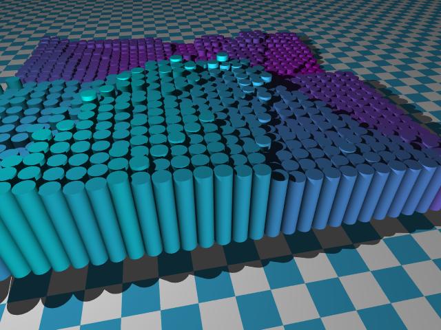
Here is a sample of the output of the fault algorithm. I used a 64 x 64 grid and then generated a set of POVRay commands to draw cylinders:
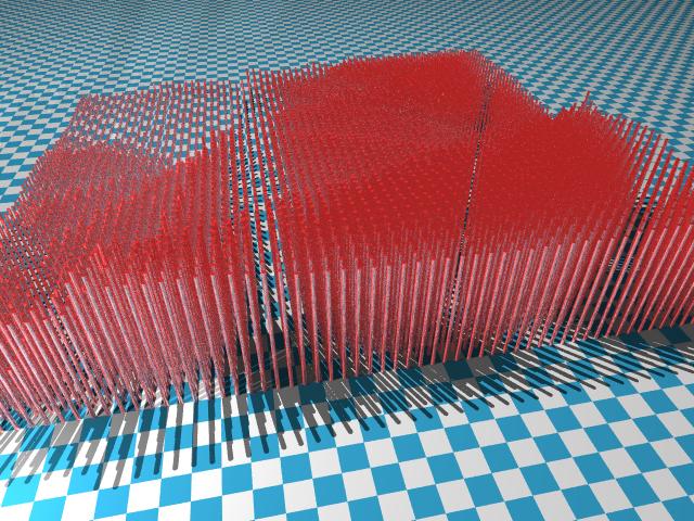
This next one is the same idea, except that the cylinders are a different colour and are much "fatter":
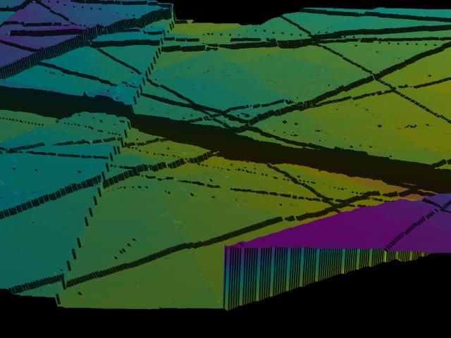
Finally, this one uses the POVRay "height_field" to read a .png file generated by the fault program: