Realtime Enough
This article appeared in Doctor Dobb's Journal, July 2007.
This article discusses the concept of “realtime enough” by way of an example, a realtime 1200 baud Bell-202 FSK modem for Caller ID, implemented under FreeBSD 5.3
As chips get faster and faster, the requirement to use a conventional “Real Time OS” (RTOS) decreases, simply due to the fact that non-RTOS (and indeed, even free) systems are “fast enough” to handle the data processing requirements. By way of example, the caller ID FSK 1200 baud modem used to be implemented in hardware, typically as a module that would accept tip and ring from the phone line on one end, and produce RS-232 on the other end. This article shows a software-only implementation of this, running on a “non realtime” free operating system.
What is Realtime?
One of my favourite interview questions is, “Define Realtime.” It's nice and open-ended, and serves as a good conversation starter. I accept pretty much any reasonable answer, but the essence of what I'm after is “something that's fast enough.”
In this article, I'm going to present portions of my voice activated call monitor which does caller ID in “realtime,” and I'll discuss how the caller ID part of the solution has evolved from a hardware FSK modem in the early 1990's through to the software FSK modem in use today. While my particular implementation is based on FreeBSD 5.3, there is nothing operating-system specific here.
First, some background. Caller ID, which is a feature that tells you who is calling, occurs as a Frequency Shift Keying (FSK) signal between the first and second ring. It operates at 1200 baud, using the Bell-202 standard which is based on 1200 Hz (a “mark,” representing a one) and 2200 Hz (a “space,” representing a zero) tones. It's a serial transmission, with a start bit, 8 bits of data, no parity, and a stop bit. At the data level, it consists of packets of information with checksums.
My hardware consists of an adaptor for a phone line:
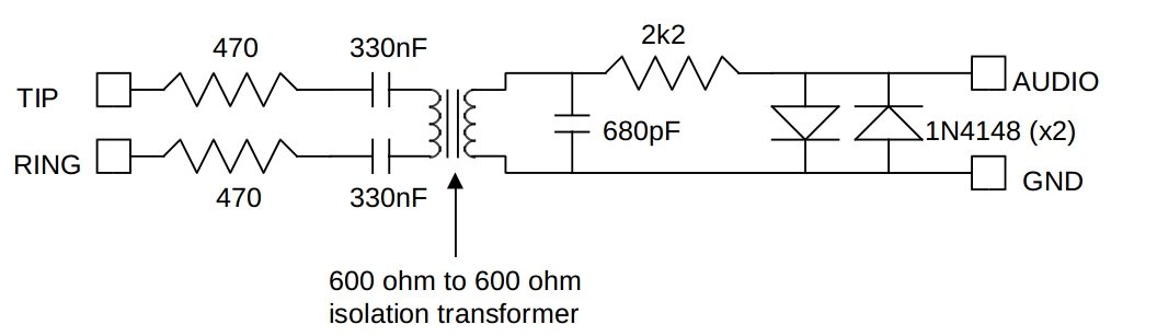
TIP and RING are the inputs from the phone line, and the AUDIO and GND are suitable to go to a line-compatible input (like a sound card). If a 600-to-600 Ohm transformer isn't available, other (similar) values will do, provided that the ratio is around 1:1. Warning: connecting this equipment to your telephone line and your soundcard is at your own risk; no warranties are expressed or implied, and all damage is your responsbility.
This converts the telephone signal into something that I can feed into a sound card's input. I have two such circuits in my system, because I have two lines. I've conveniently used the sound card's left channel for one line, and the right channel for the other.
My original requirement for the hardware was to use it as a simple, voice-activated recorder to record phone calls; later, I realized that I could do the caller ID decoding as part of the voice recorder's processing, and thus free up two serial ports (used by the hardware caller ID boxes). (Soon, I will be doing call progress tone detection and DTMF decoding, but that's currently left as an exercise for the reader.)
Here's the big picture of the system:
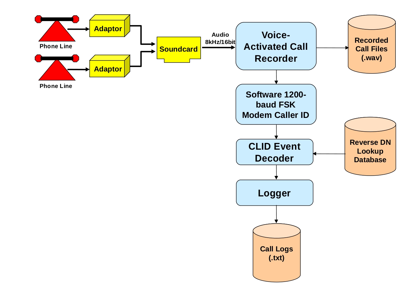
Both lines go into a sound card, and are sampled at 8 kHz. The samples then go into the voice-activated recorder, which listens for activity. When it detects activity (as defined by the signal levels going above a certain threshold, for a certain period of time), it begins recording. While it's recording, it feeds samples into the software caller ID FSK modem (there's no point in feeding samples through the modem if there's no signal).
Each sample is run through the FSK modem, and if a zero or a one is detected, the bit is then sent into a software UART (“Universal Asynchronous Receiver Transmitter,” but we're using just the receiver part). The software UART looks for the start bit, and when it gets it, accumulates eight more bits, and constructs the byte. The bytes are then accumulated in a buffer. When a sufficient number of bytes have been accumulated, the buffer is passed to the caller ID event decoder, which analyzes the buffer for caller ID information (date, time, phone number, caller's name, message waiting, etc), and stores the information. A logger is waiting for information from the caller ID event decoder, and logs the information to a text file.
Now let's look in more detail at the FSK modem part of the system, and also keep in mind the constraints affecting the realtime processing of the samples.
A sample rate of 8 kHz means that a sample arrives every 125 μs. In the past, before soundcards, an A/D (analog-to-digital) converter would simply present the digital value of the sample when the conversion was finished. This meant that something had to happen every 125 μs. The constraint here is that the system had to provide a reliable, pre-emptive scheduler, that would allow a task to be scheduled every 125 μs.
Coupled with the fact that something had to happen fairly frequently, the next issue was, how much actual work had to happen? Do you perform the FSK calculations, or do you simply buffer the data? If you buffered the data, meaning you've deferred the FSK calculations until later, then the only way you could perform the FSK work would be with a reliable pre-emptive scheduler, that interrupts your FSK calculations in order to store another sample.
However, times have changed; today's sound cards buffer the samples. This means that we don't need to worry about incurring scheduling overhead (context switches) for each and every sample. The hardware simply informs the kernel (via an interrupt) that a buffer is full and should be emptied. This then means that we can access blocks of samples, rather than being forced to get the samples one at a time from the hardware. The advantage is that we invoke a single kernel call to transfer an entire block of samples, (and then process them individually), rather than invoking kernel calls for each and every sample.
Another constraint is the actual amount of processing required to perform the FSK algorithm. If you are right on the edge in terms of CPU processing power to perform the calculations, then adding context switching overhead is not going to help. By eliminating (or vastly reducing) one constraint, you've bought yourself more time to perform the FSK work. How much work is it? Let's look at the FSK algorithm itself.
Mathematically speaking, we are constructing the following:

The gist of the above formula is that we take the sum of the square of each sample multiplied by the sine at the mark frequency for that sample step. We do the same for the cosines. We then add those two sums together for the marks, and compare them to similarly derived sums for the spaces. Whichever set turns out to be bigger indicates which tone we've detected.
In order to detect 1200 Hz and 2200 Hz tones, we construct a “correlation template.” This template is simply a table of 4 normalized (meaning that they are between -1 and +1) sets of values, giving the sine and cosine of a 1200 Hz and 2200 Hz waveform sampled at our sampling rate of 8 kHz. We only require enough samples to match the slowest waveform, which in this case is 1200 Hz. One complete waveform of a 1200 Hz sine wave, sampled at 8kHz, will require 6 2/3 samples (8000 / 1200 = 6.666...), so we can get away with just 6 samples.
So our correlation tables look like this:
| Sample | MARK | SPACE | ||
|---|---|---|---|---|
| sine | cosine | sine | cosine | |
| 0 | +0.0000 | +1.0000 | +0.0000 | +1.0000 |
| 1 | +0.8090 | +0.5878 | +0.9877 | -0.1564 |
| 2 | +0.9511 | -0.3090 | -0.3090 | -0.9511 |
| 3 | +0.3090 | -0.9511 | -0.8910 | +0.4540 |
| 4 | -0.5878 | -0.8090 | +0.5878 | +0.8090 |
| 5 | -1.0000 | -0.0000 | +0.7071 | -0.7071 |
In the sample code below, the mark waveform's sine table is at correlates [0] (corresponding to sin (θm) in the formula above), the cosine at correlates [1] (cos (θm)), the space waveform's sine table at correlates [2] (sin (θs)), and the cosine at correlates [3] (cos (θs).
// clear out intermediate sums
factors [0] = factors [1] = factors [2] = factors [3] = 0;

// get to the beginning of the samples
j = handle -> ringstart;

// do the multiply-accumulates
for (i = 0; i < handle -> corrsize; i++) {
    if (j >= handle -> corrsize) {
        j = 0;
    }
    val = handle -> buffer [j];
    factors [0] += handle -> correlates [0][i] * val;
    factors [1] += handle -> correlates [1][i] * val;
    factors [2] += handle -> correlates [2][i] * val;
    factors [3] += handle -> correlates [3][i] * val;
    j++;
}
The algorithm assumes that samples are placed into the ring buffer handle -> buffer, with the variable handle -> ringstart pointing to the beginning of the buffer.
Then, each sample in the buffer is multiplied by each of the four correlates, and the values accumulated into the factors array. (The logic dealing with j simply makes sure that j loops around the ring buffer correctly.)
The four factors correspond to the four summations in the formula given above.
So far, the total amount of work is 24 multiply-accumulates, followed by a comparison and some buffer housekeeping.
Finally, once all the multiply-accumulates are done for the four factors, we square and add the respective mark and space factors, and see which one is bigger:
handle -> current_bit = factors [0] * factors [0] + factors [1] * factors [1] > factors [2] * factors [2] + factors [3] * factors [3];
Whichever set of factors is bigger indicates which frequency was detected; therefore, if we get a true value, it means we detected a mark, else we detected a space.
The algorithm that's described above is basically a pair of matched filters at the mark and space frequencies; the result is obtained by comparing the amplitude of the output of the two filters.
Optimization
The astute reader will immediately see some optimizations that can be done.
The simplest is to eliminate the six multiplications dealing with multiply by zero, one, and negative one. This immediately saves us 25% of the multiplications!
We also have a lot of duplicate entries, so we're doing multiplication unnecessarily! Looking at the table, notice the coloured entries:
| Sample | MARK | SPACE | ||
|---|---|---|---|---|
| sine | cosine | sine | cosine | |
| 0 | +0.0000 | +1.0000 | +0.0000 | +1.0000 |
| 1 | +0.8090 | +0.5878 | +0.9877 | -0.1564 |
| 2 | +0.9511 | -0.3090 | -0.3090 | -0.9511 |
| 3 | +0.3090 | -0.9511 | -0.8910 | +0.4540 |
| 4 | -0.5878 | -0.8090 | +0.5878 | +0.8090 |
| 5 | -1.0000 | -0.0000 | +0.7071 | -0.7071 |
The red values are ones we talked about in the first optimization case (where we don't even have to do a multiplication). There are also a lot of values that are the same — but! they are for subsequent entries. Remember that each window of samples (6 samples) incurs a multiplication against the respective window member and the correlates table. We then use this to determine if we detected a mark or a space. But on the next round, we do all that work again, except one sample over. This means that we'll be multiplying against values that we already know the answer to.
We could reduce the table to:
| Sample | MARK | SPACE | ||
|---|---|---|---|---|
| sine | cosine | sine | cosine | |
| 0 | NOP | NOP | NOP | NOP |
| 1 | +K1 | +K2 | +0.9877 | -0.1564 |
| 2 | +K3 | -K4 | -K4 | -K3 |
| 3 | +K4 | -K3 | -0.8910 | +0.4540 |
| 4 | -K2 | -K1 | +K2 | +K1 |
| 5 | NOP | NOP | +K5 | -K5 |
This leaves just four “unduplicated” values, which we could gratuitously call K6 through K9 if we wanted to.
This means that we could optimize the code to do a direct assignment instead of the first sample's worth of multiply-accumulate, and then compute the individual multiplication by K1..9 and just accumulate the true or negative value.
This would mean a total of 9 multiplications (instead of 24, which is a hefty 62.5% reduction!) and 6 fewer additions. We're assuming that addition and subtraction have the same cost — accumulating a negative value (really, subtracting the value) is no more expensive.
It looks like magic...
It's hard to get an intuitive grasp of what's happening with all the multiplication and summation of sines and cosines, so here are some pictures to help illustrate. I constructed a 1200-baud FSK Bell-202 sample of the following bitstream:
010011000111000011110000011111000000111111000000011111110000000011111111
It's not a valid “CLID” bitstream, but serves to illustrate what the input looks like:

There are two values plotted in the above graph. The red line indicates the normalized (-1..+1 range) FSK audio — notice how the first 37 samples are at 2200 Hz, and the next are at 1200 Hz (I generated these at a sampling rate of 44100 Hz, so 1200 baud means each cell is 44100 / 1200 = 36.75 samples long; this is different than the 8kHz sampling we've been using throughout this article, but 44100 Hz gives a lot more samples making for a nicer plot). Also on that graph are some green lines. These are manually generated bits, indicating the bit value — the first 37 samples are shown as -1 (indicating a zero), the next are shown as +1 (indicating a one), and so on. It helps to see where the bit cell boundaries are in subsequent pictures.
Now, let's examine the effect of the summation of squares of the products of the sine and cosine correlates:
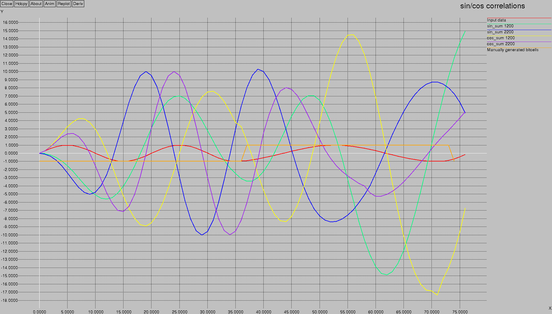
There's a lot going on in this graph! The input data is in red, and the bit cell indication is in orange; they both hover in the +/- 1 range. The first bit-cell (samples 0 to 37) is a 2200 Hz tone. Therefore, we'd expect that the 2200 Hz sin and cos product lines would be “active.” These are the blue and purple lines; indeed, you can see that during the range of the first bit-cell, the amplitudes of the blue and purple lines are maxing out at +/- 10. Interestingly, when we leave the first bit cell and move to the second one, the blue and purple lines reduce in amplitude.
Conversely, in the first bit cell we wouldn't expect much activity from the 1200 Hz correlates; and indeed the green and yellow lines have an amplitude that's smaller than they have in the second bit cell. The first bit cell limits them to around +7/-5 for the green (sin) and +7/-9 for the yellow (cos), whereas in the second bit cell they have almost double the range (+/- 15 for green and +14/-17 for yellow).
Notice that if you take the absolute values of each correlate, you'll end up with blue and purple peaks four times per bit cell for the 2200 Hz parts, and yellow and green peaks for the 1200 Hz parts.
Let's perform the final step — sum the two products and see which summation is bigger:
Wow!
The blue line clearly shows detection of 2200 Hz, and the green line clearly shows detection of 1200 Hz.
Don't worry about the slight “offset” or “delay” in the detection — this is a natural function of the fact that we have to feed several samples into the filter before it recognizes a given frequency.
The effect is a slight shift in the detection.
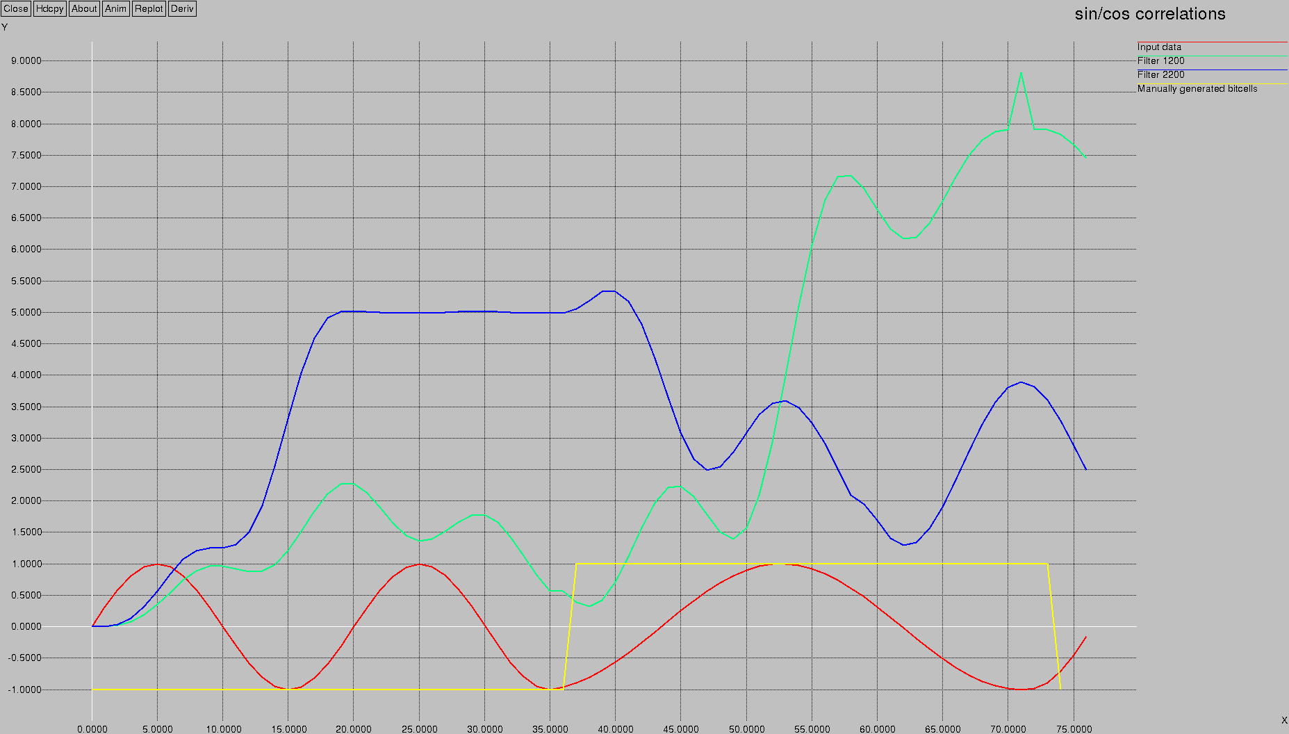
Let's look at a much bigger set of samples from the original to see that it's not a problem:

Like poetry in motion. The green versus blue shows the filter in action. (Forgive the slight mis-alignment between the yellow modulation input line and the actual sample — they were generated independently and one has a float-vs-int rounding issue accounting for the 1.8% drift :-))
Bit Cell Management
At a slightly higher level, we need to perform bit-cell management. What I mean by this is that we need to know where one bit ends and another bit starts. Obviously, if the bits have different values, this is easy: when the value changes, one bit has ended and another has started. However, what if there are several bits all with the same value, one after another? This is the topic of “clock recovery.”
Since our data stream is arriving at 1200 baud, we know that each bit cell is 1/1200 of a second long, or 833.333... μs. Next we calculate how many samples (at 8 kHz) 1/1200 of a second is. Well, this is the same number as what we came up with earlier, when we calculated how many samples we need in order to store one complete waveform at 1200 Hz. It's the value 6 and 2/3. This means that every 6 2/3 samples we have the end of one bit, and the beginning of another. However, since we are working with integral samples, it means that we have to compromise a little bit, and potentially introduce drift. (Drift is introduced not only by rounding errors, but also because your sound card will not be sampling at *exactly* 8kHz, nor will the phone company be transmitting at *exactly* 1200 baud; there will be some variation.)
The saving grace here, though, is that we are dealing with a serial protocol that has a start bit and a stop bit, which are different from each other. This means that we are guaranteed to have at least two bit reversals during an 8-bit data byte. Recall from above, that a bit reversal (a change from a mark to a space or vice-versa) tells us the definitive location of a bit cell boundary. We therefore use those for synchronization.
Here's the code that does that part:
// store previous bit in preparation
handle -> previous_bit = handle -> current_bit;

// compute current bit (as above)
handle -> current_bit = (factors [0] * factors [0] + factors [1] * factors [1] > factors [2] * factors [2] + factors [3] * factors [3]);

// if there's a bit reversal
if (handle -> prevbit != handle -> current_bit) {
    // adjust cell position to be in the middle
    handle -> cellpos = 0.5;
}

// walk the cell along
handle -> cellpos += handle -> celladj;

// gone past the end of the bitcell?
if (handle -> cellpos > 1.0) {
    // compensate
    handle -> cellpos -= 1.0;
    // tell the higher level application that we have a new bit value
    bit_outcall (handle -> current_bit);
}
The value celladj is a floating point value that indicates the fraction of a bitcell that elapses with each sample. (Yes, this could have been done with integers, but I got lazy.)
So far, we've accumulated a sequence of bits, and called bit_outcall with each bit as it arrived from the software modem.
We now need to construct a software UART; something that looks for a start bit, accumulates 8 bits, (ignores the stop bit), and calls a function to indicate that a completed data byte has arrived. Here's the code for that portion:
// if waiting for a start bit (0)
if (!handle -> have_start) {
    if (bit) {
        // ignore it, it's not a start bit
        return;
    }
    // got a start bit, reset
    handle -> have_start = 1;
    handle -> data = 0;
    handle -> nbits = 0;
    return;
}

// here, we have a start bit

// accumulate data
handle -> data >>= 1;
handle -> data |= 0x80 * !!bit;

handle -> nbits++;

// if we have enough...
if (handle -> nbits == 8) {
    // ship it to the higher level
    byte_outcall (handle -> data);

    // and reset for next time
    handle -> have_start = 0;
}
This implements a trivial state machine. The state machine begins operation with have_start set to zero, indicating that we have not yet seen the start bit. A start bit is defined as a zero, so while we receive ones, we simply ignore them. Once we do get a zero, we set have_start to a one, clear the data byte that we'll accumulate, and reset the number of bits that we've received to zero. As new bits come in, we shift them into place (using my favourite bit of obfuscated C, the “boolean typecast operator”, or !!), and bump the count of received bits. When the count reaches eight, we've received all of the bits we need to declare a completed byte, and we ship the completed data off to a higher level function (byte_outcall), and reset our have_start state variable back to zero to indicate that we are once again looking for a start bit.
If you are into such things, you could check to see that there is indeed a stop bit present. If there isn't a stop bit, you should declare a frame error in your serial transmission. I didn't bother for this application, but there is some commented-out code in the library that serves as a starting point.
At this point, we have bytes coming from a sound card -- pure magic :-) (Competent DSP engineers, however, will have fallen asleep a while ago).
What does this have to do with realtime? Well, there's a lot of computations happening:
8000 x (24 x (multiply + accumulate) + 4 x multiplies + 2 accumulates)
= 432,000 math operations per second
(to say nothing of the buffer management and housekeeping functions required).
So while I'd like to believe that I could do this on a late 1960's vintage PDP-8 minicomputer, the truth is that it would probably take at least an 8086-class processor to come close to the CPU requirements.
This ties in to the “realtime enough” aspect.
Just as certain tasks were previously completely out of the picture in terms of being done in software, so has the landscape changed in terms of “realtime” requirements. In 1993, I implemented the higher-level caller ID software, but relied on hardware FSK modems, because it was inconceivable (to me, at least) that I could do this in software. The 1993 implementation relied on a realtime OS, QNX 4, in order to make sure that the CPU got allocated to the serial port handler when data arrived, and then got allocated to the high-level caller ID software, to ensure timely processing.
Today, I run the full software caller ID package as described above on a free OS (FreeBSD 5.3) and I didn't even bother using the realtime scheduling features of the kernel. It barely uses enough CPU to show up as more than 0.00% on the CPU monitor.
It's “fast enough.”
Other Filters
Goertzel filters are another type of filter; I'll write an article one day about them. But for now, ever wonder what those tones were at the end of Pink Floyd's “Young Lust?” You know the ones, after the operator asks, "Do you accept the charges from the United States?" The guy hangs up, you hear 2600 Hz to clear the line, and then:
Those are MF tones (for Multi-Frequency). And, using a Goertzel filter, they magically decode to the sequence: KP 0 4 4 1 8 3 1 ST. Now you know.
References
For an excellent book on DSP, I highly recommend Richard G Lyon's book, ISBN-0131089897, “Understanding Digital Signal Processing”, published by Prentice Hall. Richard explains and demystifies DSP.
When I get around to understanding how the algorithm works, I should consult More on Product of Sines and Cosines.