Here a mole, there a mole, everywhere a mole!

Counting Moles

Moles are like fingerprints; you can find constellations of moles almost anywhere — on your back, your arms, legs, face. But writing software to track them is not as easy as it sounds. In this article, I'll look at what it takes to write software that can extract moles from pictures, and then track them between images taken at various time periods.

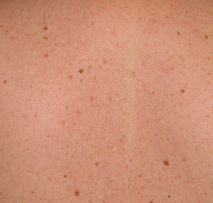
First, some pictures. This is a small section of a back, showing a variety of moles:

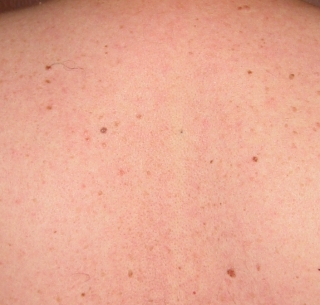
Two weeks later, another picture:

As you might imagine, it's desirable to be able to spot any new moles, or changes in shape of existing moles. So, here they are side by side:

As you can guess, there are going to be a few challenges:

• different lighting (the second mole set is brighter)
• different view (the second mole set was taken slightly higher than the first)
• different angle (some slight variation in camera angles is likely to happen)
• variations in skin colour

In the first part of the development of my program kmole, I'm interested in detecting new moles.

The approach I've taken is to try and identify the major moles and have the program use them as a map to figure out where the moles should be in relation to one another. The first step, therefore, is to come up with an algorithm that detects moles.

I tried various methods, such as sum of squares of differences and triggering when a threshold was detected, or comparing against a well-defined colour (and triggering on a threshold), but the method that seems to work best is an average discrepancy filter.

The average discrepancy filter works by taking an area of pixels, say 30 x 30 (900 pixels) around a given centre pixel, and computing the average colour for that block. Then, the centre pixel is compared against the average, and if it's different from the average value by a certain threshold, it's tagged.

This is what the average colour filter is working with:

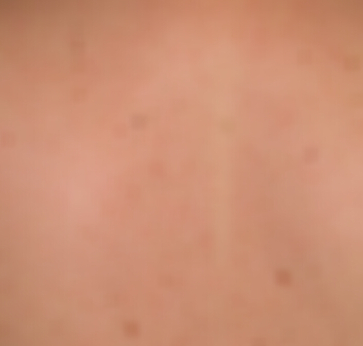
This does what you'd intuitively expect — it effectively blurs the image. But it does so in a “square” way — notice how the moles look like they are square instead of round. That's because I used the following algorithm:

for (int y = 0; y < h; y++) {
    for (int x = 0; x < w; x++) {
        int numpoints = 0;
        double  r = 0, g = 0, b = 0;
        for (int ix = -XSIZE; ix < XSIZE; ix++) {
            if (x + ix >= 0 && x + ix < w) {
                for (int iy = -YSIZE; iy < YSIZE; iy++) {
                    if (y + iy >= 0 && y + iy < h) {
                        r += image.r (x + ix, y + iy);
                        g += image.g (x + ix, y + iy);
                        b += image.b (x + ix, y + iy);
                        numpoints++;
                    }
                }
            }
        }
        if (numpoints) {
            r /= numpoints;
            g /= numpoints;
            b /= numpoints;
        }
        average.value (x, y, { (int) r, (int) g, (int) b });
    }
}

Effectively, I coded a square grid of 2 x XSIZE by 2 x YSIZE. A more effective algorithm, which I'm going to explore, is to come up with a list of (x, y) points and use those. The nice thing about that is that the list can be generated as a thick circle; excluding some number of pixels in the centre, and including only pixels between an inner and outer radius. (If you're particularly clever, your list of (x, y) points can actually be a list of (x, y, weight) points, allowing you to specify custom weighting for averaging.) If the list was presented as a vector<xy>, it could be done like so:

...
for (auto &xy : vlist) {
    if (x + xy.x >= 0 && x + xy.x < w && y + xy.y >= 0 && y + xy.y < h) {
        r += image.r (x + xy.x, y + xy.y);
        g += image.g (x + xy.x, y + xy.y);
        b += image.b (x + xy.x, y + xy.y);
        numpoints++;
    }
}
...

Effectively replacing the inner X and Y block with a custom list called xy (a struct with two members, x and y).

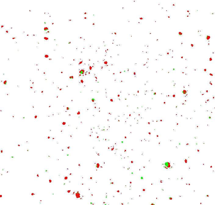
Now, computing the discrepancy against a threshold yields an interesting result:

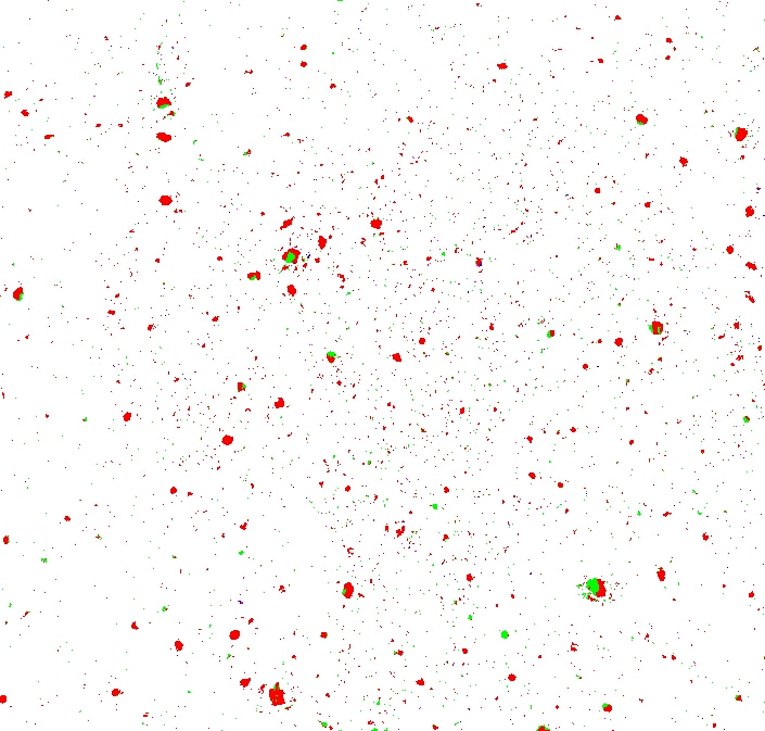
Some pixels are red (when the red channel's discrepancy was greatest) and some are green (when the green channel's was greatest) — there are no blue pixels (the blue channel's discrepancy was never greater than either of the red or green channels').

There's a lot of noise in the image — places where only a few pixels are considered different, giving the image a “speckly” look. We can eliminate that by counting neighbours. The algorithm is simple: if a given pixel has fewer than one or two neighbours, we kill it. Much better:

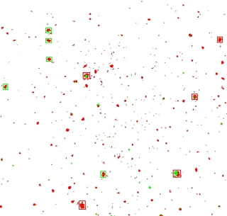
The next step in the process is to sort the moles by size. I used a really cheesy algorithm and simply gave each pixel that was not white (so the red and green ones) a unique value. Then I “joined” all the neighbours, effectively coalescing them into clumps. I sorted the results by the number of pixels involved, and marked the top 5 clumps with a red square, and the next top 5 with a green square.

If you now compare this side-by-side with the second original picture, you'll see that we have the basis for comparing the major mole constellations:

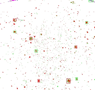Improvements planned for the next coding session are:

• mark all features greater than a certain size (not just the top N)
• compute shortest-distance to neighbours
• compute angle between neighbours
• create a database of moles and { distance, angle } pairs
• correlate one picture with the next.

Stay tuned as more developments take place.