Implementation notes for a C++ stock analysis library
Following on to my The Design and Development (and Performance) of a Simple Trading AI article, I spent a few days improving my library for dealing with stock data. The previous library was C-based and mmap'd in a huge (700MB) data file complete with pointers and all!
I figured there needed to be a C++ library that dealt with higher level concepts on top of the raw database implementation provided.
So I wrote one.
C++ and Graphs Digression
Let me digress (quickly) about the power of C++. (Yes, I'm like an ex-smoker — I realize that!) In C, doing the below graphs would have taken a significant amount of effort. In C++, I whipped these out in a matter of an hour or two. Let's revel in the beauty of these graphs first before talking about the C++ library:
The first graph shows a distribution of correlation values for various stocks using the sum of squares of errors method. What I mean by that is that I went through my database of 260 stocks (all the optionable stocks on the TSX) and compared each stock to every other stock. I was hoping to see which stocks behaved the same as other stocks.
Doing on the order of 2602 comparison operations over a year's worth of data, I came up with the following graph:
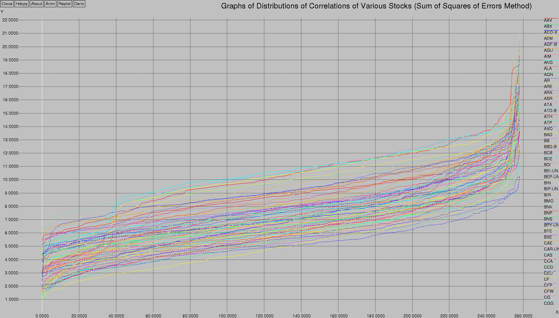
It shows the top-most values obtained from all that data — for each stock (each line), what is the correlation with each stock (on the X axis)? The results are sorted.
So, taking the first (bottom-most) yellow line (representing the correlation to the stock called “AAV”), at X=0 the value (5.47) represents the sum of squares of errors between this stock and some arbitrary stock in the database. The second value, X=1 (5.84), represents the sum of squares of errors between this stock and some other arbitrary stock in the database. The sum of squares of errors is sorted in ascending order. The last (highest, most non-correlated) stock at X=258 (18.70) represents “AAV”'s correlation to its most non-correlated stock.
This ends up giving us a nice smooth line like the one you see above, for each stock (I could only fit a little over 80 stocks on the graph before xgraph barfed).
What's interesting is the general shape of the graph — there's a bit of a ramp at the first 40 samples, then it flattens out, and then there's another ramp at around 240. What's that all about?
Using the power of xgraph, I captured the 1st derivative of these values:
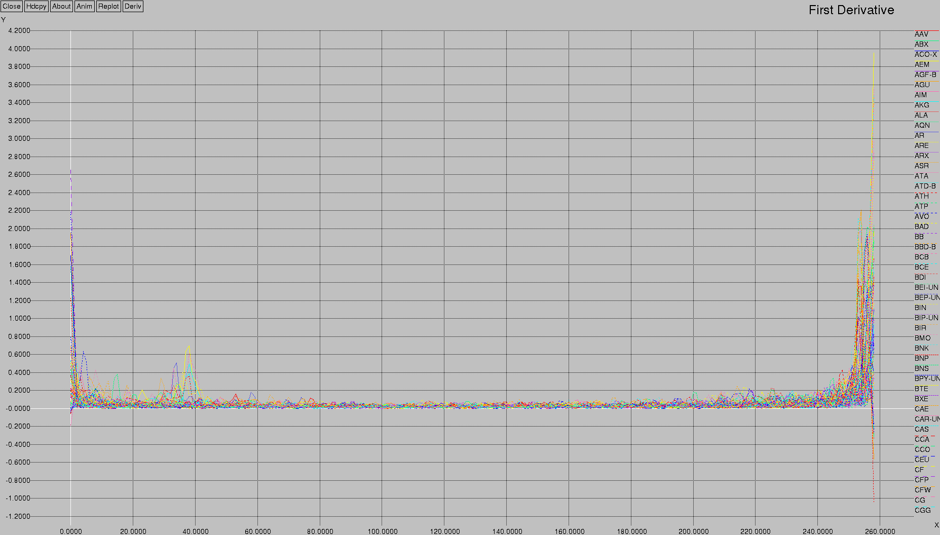
This quite clearly shows what's going on with respect to the distribution of values — there's a clustering at the first 10, and then another one at around 35-40, and then nothing until the end.
This clustering is useful in order to help cluster the individual stocks. Just like neurons (“neurons that fire together, wire together”), stocks that are highly correlated will behave similarly. This is a useful datapoint for future work.
The above was done with a “sum of squares of errors” model. This means that I compare, element-by-element, two stocks. I compare their normalized (normalized to the closing price) change from the previous day. I take the difference between their two values and square it, and then add the result to the sum. The output is the sum of the difference of the errors.
That's what you see in the charts above.
You could take a simpler approach. You could simply say if the stocks go in the same direction, they get a +1, otherwise they get a -1. So, if the two stocks you're comparing both go up on the given day, add one to your score. If they both go down, add one. If they go in different directions, subtract one. After a year's worth of data has been analyzed, return the sum of the results.
I call this the “Boolean Method” in that it takes into account just a binary value — it doesn't care how much of a change there was in the stock value, just that the change was in the same direction for both stocks.
This is what that looks like, if plotted using the same algorithm as above:
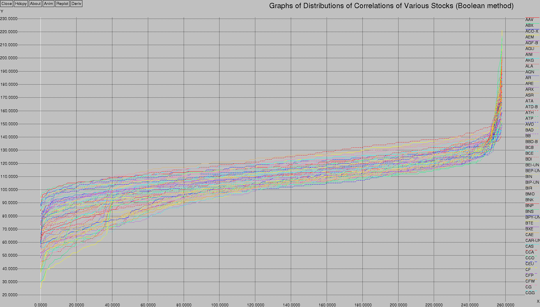
Interesting, eh?
The centre channel is thinner, and, while there are still two bands of correlation activity (0-10 and 35-40), the shapes are a little bit different.
Here's what the 1st derivative looks like:

We may return to more detailed analysis of these graphs in a future article; they serve as a “here's what I need to be able to do easily with this library” use case.
Library Operations
For the kinds of financial analysis I want to do, I need to be able to generate lists of data points.
I have five basic classes for the stock library:
- a Stock base class,
- an Equity and EquityData class for equities, and
- an Option and OptionData class for options (derivatives).
So, to get a list of the last year's worth of data for my favourite stock, the Bank of Nova Scotia (“BNS” on the Toronto Stock Exchange):
Equity bns (YMD {} - 365, "BNS");
This constructs an object called bns that contains the requisite data set. (I have a private class called YMD that takes dates, or as shown above, defaults to “today.” It has overloaded plus and minus operators so that you can go forward and backwards in time, like I did by subtracting 365 days.)
The constructor for Equity is overloaded and defaulted, I could have equivalently written the above as any one of:
Equity bns (YMD {2014,8,16}, "BNS", 250);
Equity bns (YMD {2014,8,16}, "BNS", YMD {2015,8,16});
The magic constant 250 assumes that there are 250 records that I want to retrieve; it's much better to let it default to the second, date based form, where the defaulted parameter is “today.” But it does give you the flexibility of asking for January 2012's data, for example:
Equity bns (YMD {2012,1,1}, "BNS", YMD {2012,1,31});
To dump out the closing prices for that data set:
cout << "BNS closing prices (year to date)\n";
for (auto i : bns) {
    cout << i.date() << " " << i.close() << "\n";
}
Easy peasy, as I like to say.
The Stock base class is used to do things over the entire database, like list all the available exchanges and stocks:
vector <string> exchanges = Stocks().list_exchanges();
vector <string> equities = Stocks().list_equities();
(Yeah, I should probably modify list_equities to take an exchange; let's just pretend that it defaults to the TSX).
Generating Graphs
Tying this all back to the pretty graphs I generated above, the main correlation database was created as follows. First, I get a list of all the stocks available:
int
main (int argc, char **argv)
{
...
    // create a matrix of all stocks [STOCKS x DATUM]
    vector <string> names = Stocks().list_equities ();    // [STOCKS x 1]
    vector <Equity> matrix;                               // [STOCKS x DATUM]
    for (auto i : names) {
        matrix.push_back (Equity (YMD {} - 365, i));
    }
...
Next, I calculate the changes from one day's close to the next's. I also normalize those values so that they are all in the range 0..1
    // normalize the delta close (change) values (range 0..1)
    cout << "Normalizing " << names.size() << " entries\n";
    vector <vector <double>> changes (names.size(), vector <double> (largest, 0));    // [STOCKS x DATUM]
    for (int row = 0; row < names.size(); row++) {
        double previous = matrix [row][0].close();              // initialize "previous" value
        double lowest = matrix [row][1].close() - previous;     // lowest and highest are the first values
        double highest = lowest;
        changes [row][0] = 0;                                   // initialize to sane value
        for (int column = 1; column < largest; column++) {
            changes [row][column] = matrix [row][column].close() - matrix [row][column - 1].close();
            if (changes [row][column] < lowest) lowest = changes [row][column];
            if (changes [row][column] > highest) highest = changes [row][column];
        }
        if (highest == lowest) highest++;                       // if they are the same, keep the lowest as a lower bound and make the delta be 1
        // renormalize so that they all have the same range
        for (int column = 1; column < largest; column++) {
            changes [row][column] /= highest - lowest;
        }
    }
And finally, I correlate the stocks, each stock against the other. I do that by creating a really nasty looking structure: vector <tuple <double, string, string>> called correlations. This is the list that I fill as I evaluate each stock versus each other stock. I push_back the computed correlation, along with the names of the two stocks by way of make_tuple.
...
    // correlate them one against each other
    vector <tuple <double, string, string>> correlations;   // [2xSTOCKS x 1]

    for (int co_row = 0; co_row < names.size(); co_row++) {
        for (int co_column = co_row + 1; co_column < names.size(); co_column++) {
            double c = correlate (changes [co_row], changes [co_column]);
            correlations.push_back (make_tuple (c, names [co_row], names [co_column]));
        }
    }
That's all there is to it. Granted, some of it is a little dense, especially when we get to the two dimensional matrices and the tuples.
By the way, this is the correlate correlation function:
static double
correlate (vector <double> a, vector <double> b)
{
    if (a.size () != b.size()) {
        throw (runtime_error ("correlate (a (size " + to_string (a.size()) + ") != b (size " + to_string (b.size()) + "))"));
    }

    double  sum_errors_squared = 0;

    for (int i = 0; i < a.size(); i++) {
//      sum_errors_squared += (a [i] - b [i]) * (a [i] - b [i]);
        sum_errors_squared += (a [i] < 0 && b [i] >= 0) || (a [i] >= 0 && b [i] < 0);
    }
    return (sum_errors_squared);
}
The commented out code just selects between sum of square of errors versus Boolean, it's currently set to Boolean.
Finally, the data is sorted (via a handy little lambda function) and written to standard output where xgraph can display it:
    // sort by first stock and then correlation
    sort (correlations.begin(), correlations.end(),
    [] (tuple <double, string ,string> const &a, tuple <double, string, string> const &b) {
        if (get <1>(a) == get <1>(b)) {
            return (get <0>(a) < get <0>(b));
        }
        return (get <1>(a) < get <1>(b));
    });

    cout << "\n+XGraph snippable data sets\n";
    cout << "Title \"Correlation Map\"\n";
    string last = "";
    int     x = 0;
    for (auto i : correlations) {
        if (last != get<1>(i)) {
            last = get<1>(i);
            cout << "\n\"" << last << "\"\n";
            x = 0;
        }
        cout << x << " " << get <0>(i) << "\n";
        x++;
    }
So, let's return to some more graphing functions, shall we?
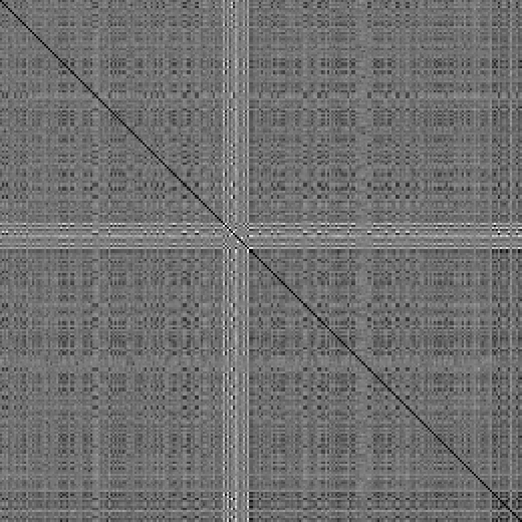
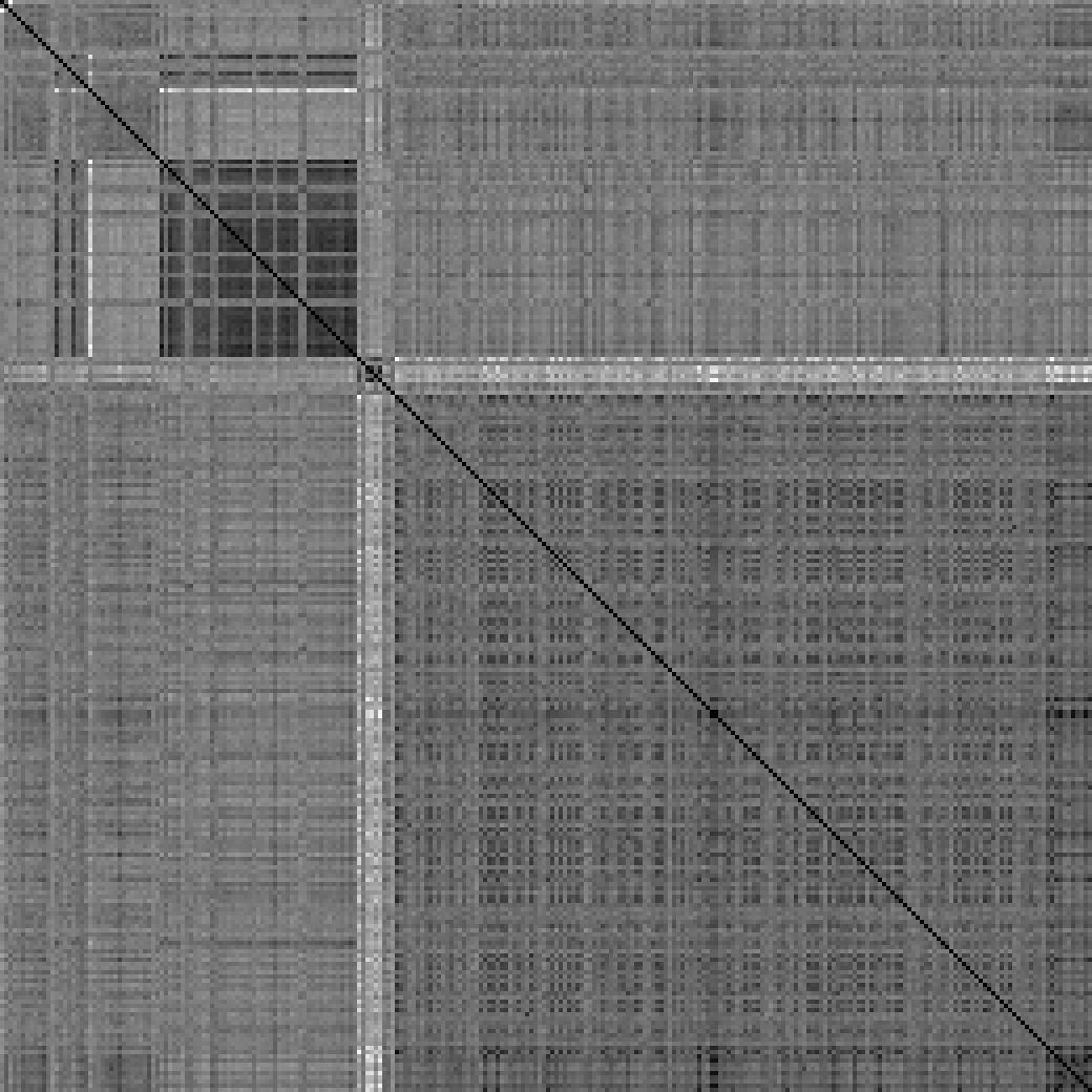
Using the Sum of Squares of Errors method, we arrive at the following correlation matrix (sorted by stock name on both axes):

And compare with the Boolean method:
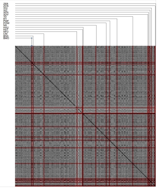
Annotating the Boolean method for bank and financial stocks:
Clustering
I took a really cool course from coursera.org called “Mining Massive Data Sets” (taught by Leskovec, Rajaraman, and Ullman) — I'll just call it MMDS here.
In it, Dr. Leskovec talked about how to take an adjacency matrix and use it to create clusters of data.
This is what that looks like, for both the Boolean one:
And the sum of square errors one:
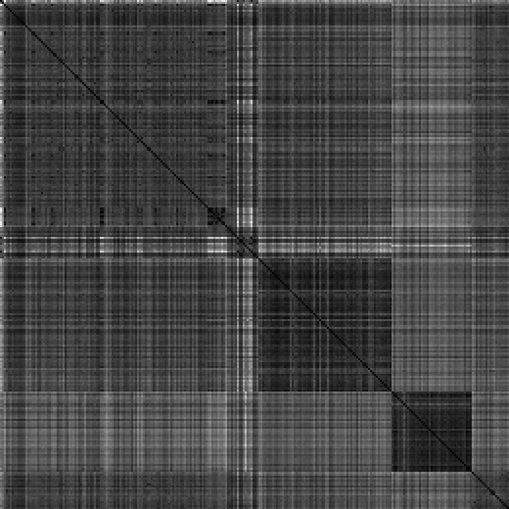
This is with 5 seed clusters.
Algorithms
Doing all of the graphing and correlation work above, I found myself doing the following operations:
- dealing with the list of stocks (as strings and indices into the names array)
- creating vectors and matrices (all kinds, but mostly STOCKS x DATUM or STOCKS x STOCKS in shape)
- sorting
Let me first digress a little and talk about the algorithm I used for sorting the adjacency matrix. In the MMDS course, the method they used to “sort” the matrix so that clustering became apparent involved Eigenvectors and other complicated math. My approach is much simpler:
- determine the number of clusters (“seeds”) that you want (say 10).
- pick the two stocks that have the highest dissimilarity; these are your first two seeds.
- while there are more stocks to pick:
- pick a stock that has the most dissimilarity to all existing seeds
- add that stock to the seed list
- Now that all the seeds have been picked, go through all the remaining stocks and see which bin (“seedbank”) they go into and put them there.
The choice of the two initial stocks is actually somewhat predictable — it ends up being two ETF's that track the S&P-60; one tracks true (HXU) and one tracks inverse (HXD), so of course they're going to be anti-correlated.
The intuition about the algorithm is that the clusters should be based around things that are dissimilar. So picking an initial set of seeds for the cluster based on dissimilarity seemed like a good idea. The seedbank idea, that is, fitting the remaining stocks into each of the (now fixed) seed bins, is currently done based on comparing each stock against one of the N seeds (“seed heads”) and simply dropping it into the best-fit seedbank.
My seedbank, using the Boolean method, was:
| Stock | Name | Score | Comment |
|---|---|---|---|
| HNU | HorizonsBetaPro NYMEX Natural Gas Bull+ ETF | 123 | Initial seeds |
| HND | HorizonsBetaPro NYMEX Natural Gas Bear+ ETF | 123 | Initial seeds |
| ABX | Barrick Gold | 125 | |
| HGD | HorizonsBetaPro S&P/TSX Global Gold Bear+ ETF | 155 | |
| HGU | HorizonsBetaPro S&P/TSX Global Gold Bull+ ETF | 132 | |
| GIB-A | CGI Group | 128 | |
| HXD | HorizonsBetaPro S&P/TSX 60 Bear+ ETF | 134 | |
| HXU | HorizonsBetaPro S&P/TSX 60 Bull+ ETF | 133 | |
| HIX | HorizonsBetaPro S&P/TSX 60 Inverse ETF | 129 | |
| XIU | iShares S&P/TSX 60 | 128 | |
| HFD | HorizonsBetaPro S&P/TSX Cap F Bear+ ETF | 128 | |
| ZEB | BMO S&P/TSX Equal Weight Banks ETF | 129 | |
| BTE | Baytex Energy Corp. | 125 | |
| HED | HorizonsBetaPro S&P/TSX Cap E Bear+ ETF | 132 | |
| TOG | TORC Oil & Gas Ltd | 126 | |
| HOD | HorizonsBetaPro NYMEX Crd Oil Bear+ ETF | 127 | |
| SVY | Savanna Energy Services Corp | 126 | |
| XSB | iShares Canadian Short Term Bond | 125 |
13 of the 18 stocks are ETFs or other “artificial” stocks. Interesting. Half of the ETFs are understandable — Horizons Beta Pro offers both “bear” and “bull” ETFs. The bull ETFs are true, the bear ETFs are inverse, so once you've got one it's inevitable that you'll get the other. If you refer back to the adjacency matrices above, there's usually a white cross pattern readily apparent. White indicates an area of least correlation. You'll notice something about the Horizons Beta Pro offerings — they all start with the letter “H,” which means that in the unsorted adjacency matrix they'll all be near the middle. Pattern spotted.
My populated seedbank, from the above, is as follows (this is what gets plotted, effectively):
| Symbol | Count | Content |
|---|---|---|
| HND | 0 | |
| HNU | 0 | |
| ABX | 2 | NGD, S |
| HGD | 0 | |
| HGU | 37 | AEM, AKG, AR, ASR, CG, CGG, CGL, CNL, DGC, DPM, EDR, ELD, FNV, FR, FVI, G, GUY, IMG, K, KGI, NG, P, PAA, PG, PVG, RGL, RMX, SEA, SLW, SMF, SSL, SSO, SVM, THO, XGD, XMA, YRI |
| GIB-A | 12 | BCB, BCE, BPY-UN, CAS, CGX, OTC, POT, QBR-B, RCI-B, TCN, U, XIT |
| HXD | 0 | |
| HXU | 86 | ACO-X, AGF-B, AGU, AIM, ALA, ARE, ATA, ATP, AVO, BBD-B, BEP-UN, BIN, BIP-UN, CAE, CAR-UN, CCO, CF, CFP, CIX, CLS, CNR, CP, CPX, CTC-A, CU, CUF-UN, CUM, DDC, DH, DOL, DRG-UN, EFN, EMA, ENB, ENF, FCR, FM, FTT, GEI, GIL, GMP, GRT-UN, HNL, HXT, IAG, ITP, KEY, MNW, MX, NBD, NPI, PKI, POW, PPL, PWF, RBA, REI-UN, RFP, RUS, SLF, SNC, SOY, SPB, STB, STN, SU, SW, TA, TCK-B, TCM, TFI, TIH, TRI, TRP, UFS, WFT, WIN, WJX, WSP, WTE, X, XDV, XIC, XSP, XSU, ZCN |
| HIX | 0 | |
| XIU | 26 | ATD-B, BB, BEI-UN, CCA, CSH-UN, EMP-A, EXE, FTS, HBC, IFC, IGM, INE, JE, MFI, MIC, MRE, NSU, OCX, REF-UN, SJR-B, T, VRX, VSN, WN, WPT, XIN |
| HFD | 0 | |
| ZEB | 19 | AQN, BMO, BNS, CM, CWB, GC, GWO, HCG, HFU, IPL, MRU, NA, PJC-A, RON, RY, TCL-A, TD, WJA, XFN |
| BTE | 29 | BDI, BNP, BXE, CNQ, COS, CVE, ECA, ERF, ESI, FRU, GTE, HBM, HEU, HSE, LIF, LTS, PD, PGF, POU, PRE, PSI, PWT, SCL, SCP, TCW, TDG, TET, VET, XEG |
| HED | 0 | |
| TOG | 29 | AAV, ARX, ATH, BAD, BIR, BNK, CEU, CFW, CJR-B, CPG, CR, CS, EFX, FRC, IMO, KEL, MEG, MTL, NVA, PEY, PPY, PXT, RRX, SES, SGY, TGL, TOU, WCP, WRG |
| HOD | 0 | |
| SVY | 1 | CUS |
| XSB | 1 | XCB |
Canada's top 5 banks (BMO, BNS, CM, RY and TD) some smaller banks (CWB, NA), and an ETF (XFN), all highlighted in red, correlate to the seed head “ZEB” (the BMO S&P/TSX Equal Weight Banks ETF), so that's a good sign that the algorithm is working :-)
Mining companies, predominantly gold and silver, are highlighted in blue on the seed head “HGU” (the HorizonsBetaPro S&P/TSX Global Gold Bull+ ETF), so that's another good indication. Barrick, “ABX,” didn't make the list — it got its own seedhead and two friends (NGD (Newgold Inc) and S (Sherritt International)) but didn't attract any other followers.
It may be useful to refine the algorithm a little bit, by comparing the candidate stock against all stocks in each seedbin, and see which seedbin it fits into. If that's the case, then it might also make sense to compare all remaining stocks against all stocks in each seedbin, and populate the seedbins one candidate stock (best fit) at a time. I haven't played with those modifications to the algorithm yet.
A further refinement would be in the seedhead selection. Notice that the seedheads with zero entries are predominantly inverse ETFs (they start with “H” for Horizons Beta Pro and end with “D” for “Down” (as opposed to “U” for “Up”), to wit: HND, HGD, HFD, HED, and HOD). XSB (Short term bond ETF) correlated to XCB (Corporate bond ETF), and nothing else. Weird.
One clever hack I did was instead of figuring out how to sort a 2D matrix (the rows would be easy, it's the columns that are a pain) I simply used a translation vector to pick out the entries in sorted order.
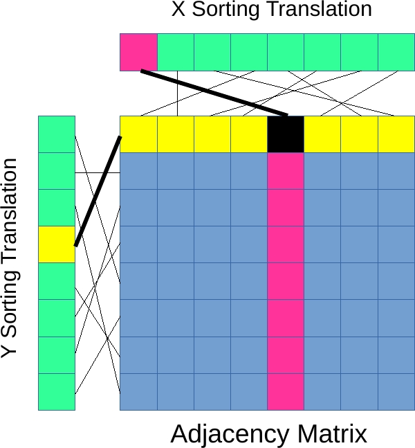
In the diagram above, the location (0, 3) is shown. The X value (0) is converted to the actual sorted X value (4), and the Y value (3) is converted to the actual sorted Y value (0), giving the location of the black square (4, 0). So (0, 3) → (4, 0).
And now, a false colour image out of the latest version:

This was made by normalizing the correlation factor to the 0..1 range, and then:
unsigned int r = 128. + sin (normalized * 4.) * 128.;
unsigned int g = 128. + sin (normalized * 40.) * 128.;
unsigned int b = 128. + sin (normalized * 400.) * 128.;
Let's call the above {4, 40, 400}.
Even more spectacular results can be obtained by bumping up the frequency:


The above was generated using {200, 201, 199} — very close “beat” frequencies, if you like.